
It might be tricky to coordinate data transfer between CAD and GIS application, but there is at least one easy way this tutorial will walk you through. It will briefly touch necessary concepts for understanding the difference between CAD and GIS application and show the example of one-way data flow.
You can also watch a more detailed Youtube tutorial.
The setup for this tutorial is:
- a Speckle account (you can get one at https://speckle.xyz/)
- QGIS 3.16.13, plugins: QuickOSM 2.0.0 (QGIS->Plugins->Manage and Install Plugins)
- Speckle Connector for QGIS (QGIS->Plugins->Manage and Install Plugins, follow the installation guide)
- Rhino 6 & Grasshopper
- Speckle Connector for Grasshopper (install it via Manager)
Importing raster data
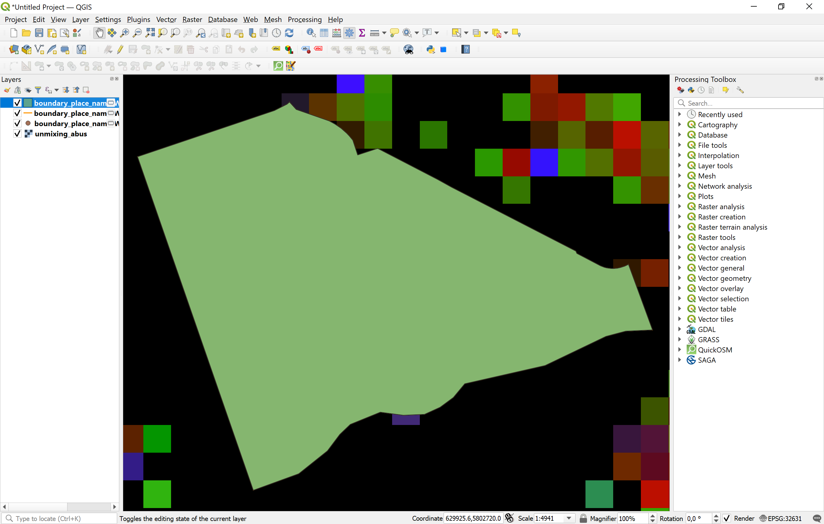
One of the data types we will work with is raster data, untypical for CAD but widely used in GIS. Raster data is made up of pixels/cells each containing a value, and can serve as a background containing contextual information, or for visualizing spatial phenomena (e.g. continuous - elevation, population density, or discrete - land use etc.). The data for this tutorial is a vegetation cover downloaded from EOC Geoservice of the Earth Observation Center (EOC) of the German Aerospace Center (DLR) under "fCover Sentinel-2 Netherlands" dataset. The downloadable folder containing data for Amsterdam is "31UFU_20160908", and the file is "unmixing_abus.tif". You can check the Readme file for details of the dataset. Drag the file to the layers of the newly created project in QGIS:
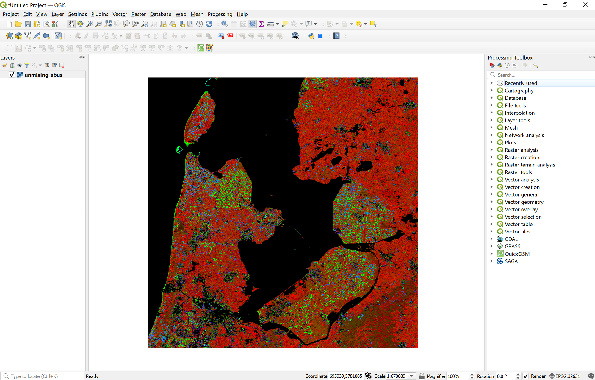
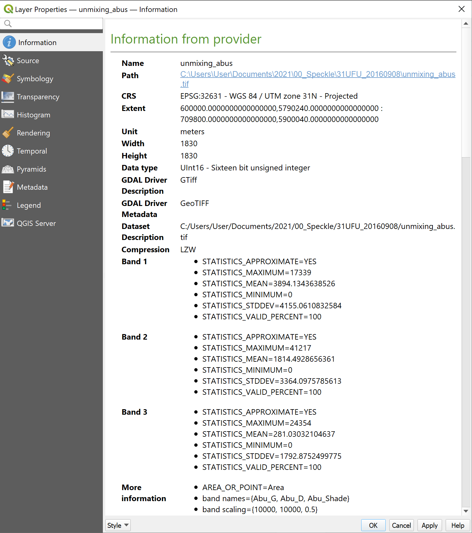
Double-click on the layer name to open Layer Properties. Information tab describes the data contained within the layer, in our case we have a multi band raster with 3 bands (or, attributes), and from the Readme file we know that we need band 1 "Abu_G" showing photosynthetically active vegetation (PV).
Second important thing we can see in the layer properties is Coordinate Reference System (CRS). They can be of two types: Geographic Coordinate Systems and Projected Coordinate Systems. The main thing to keep in mind here: for use in CAD we will need the coordinates to be stored in linear units (i.e. meters rather than degrees), therefore the Project CRS should be stored set as a projected coordinate system. The layers' individual CRSs (the way data is stored for each layer) can be any, as Speckle connector will reproject it to the global Project CRS before sending.
Tip: you don't see the discrepancies in different layers' coordinate systems because of the QGIS function "on the fly" CRS that automatically adapts all layers to your Project CRS (shown in the bottom right corner of the QGIS window), so all the layers are rendered in the correct position in relevance to each other. Rhino doesn't know how to treat different coordinate systems, so we need to prepare the data before sending.
Importing OpenStreetMaps data
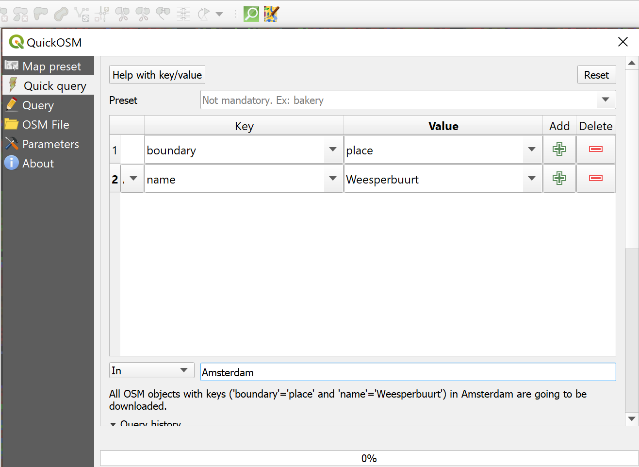
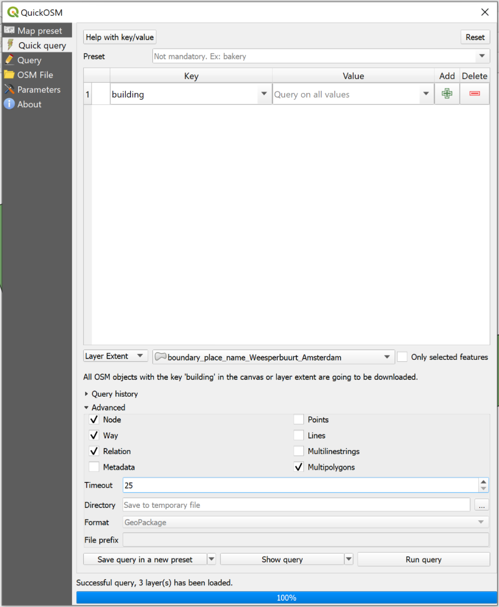
Let's leave the raster layer for a moment. To get more a specific boundary of our location of choice we will activate QuickOSM plugin with inputs from the image below, and click Run query on the bottom of the same pop-up window.
Tip: to select the keywords for query, I usually go to OpenStreetMaps, zoom to the chosen location, right-click->Query features. From the list of nearby or enclosing features you can click on the one you need and check the details.
Tip #2: by default, new layers will be saved as Temporary layers with a chip-icon next to it. You can click on it to save the layer to file, otherwise it will not be accessible after closing the project.
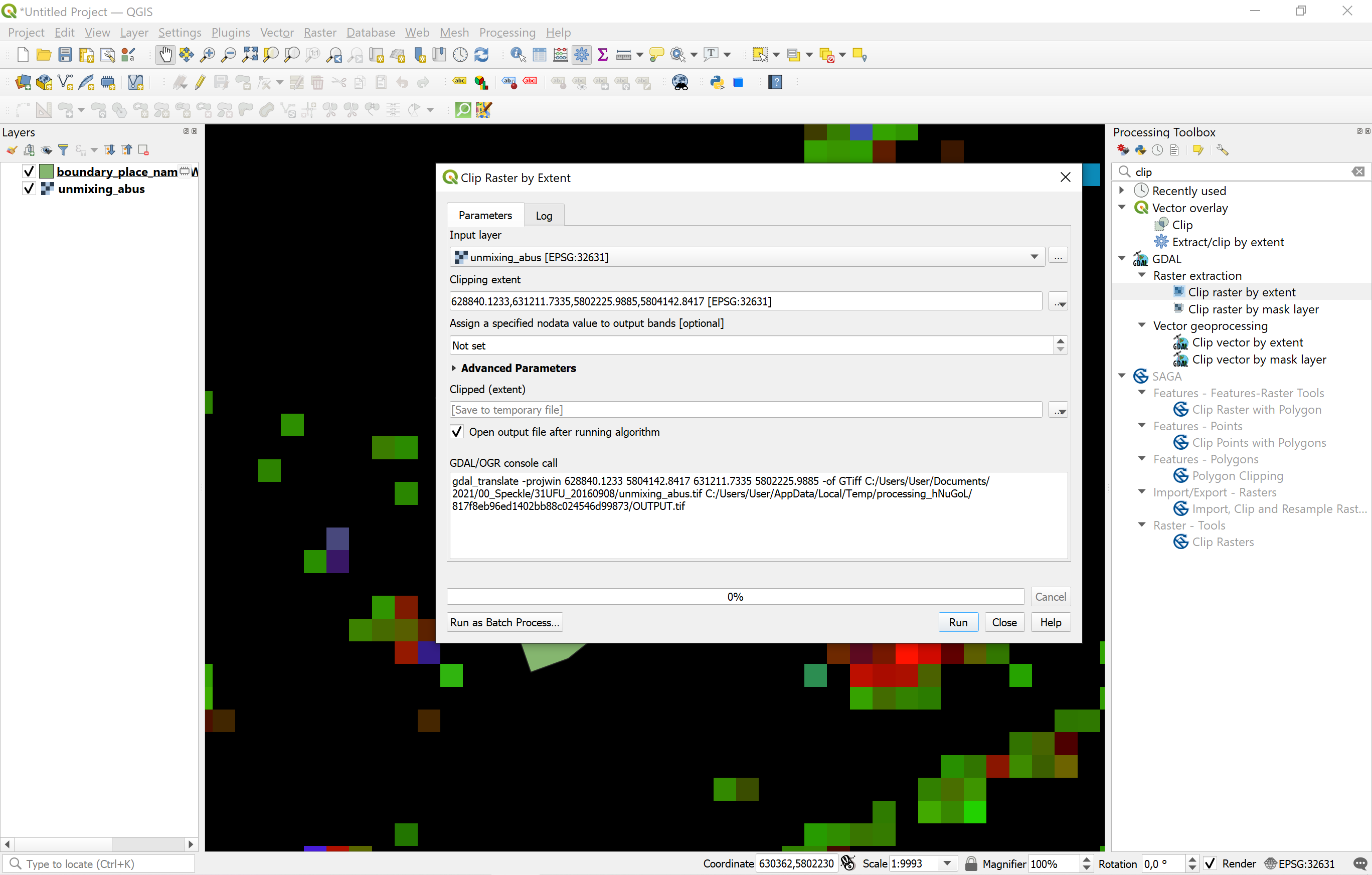
Clipping the layer
Right-click on the newly created polygon layer->Zoom to Layer. You can delete the Point and LineString layers.
In the Processing Toolbox find Clip raster by extent, double-click. Set the Input layer and Map Canvas extent and click Run. You might want to zoom out slightly to get more data around the border of your area. You might not want to clip raster by the boundary itself, as in the further analysis you will get a strong border effect close to the boundary. Clipping by Map Canvas extent gives enough buffer to avoid it.
If you don't see the Processing Toolbox, right-click somewhere on the panel and set the checkbox for Panel ->Processing Toolbox Panel.
Sending layers with Speckle
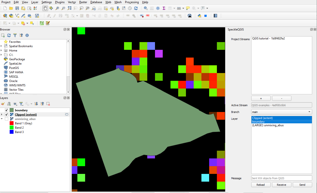
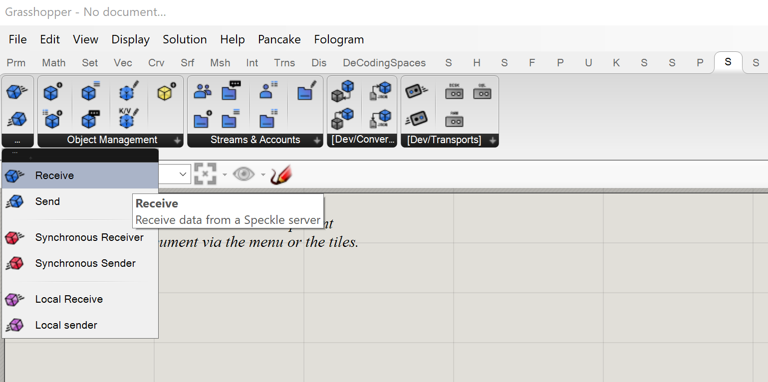
Finally, let's use Speckle connector! If you activated the plugin, you will see a beautiful blue brick in plugins toolbar, click on it to open the toolbar (make sure you logged in via SpeckleManager desktop app). Select layers for sending, set the URL (or just id) of the stream where you want to send the data and click Send.
Tip: if you renamed the layer after creation and don't see the new name in Speckle layer list, click Reload to refresh the list.
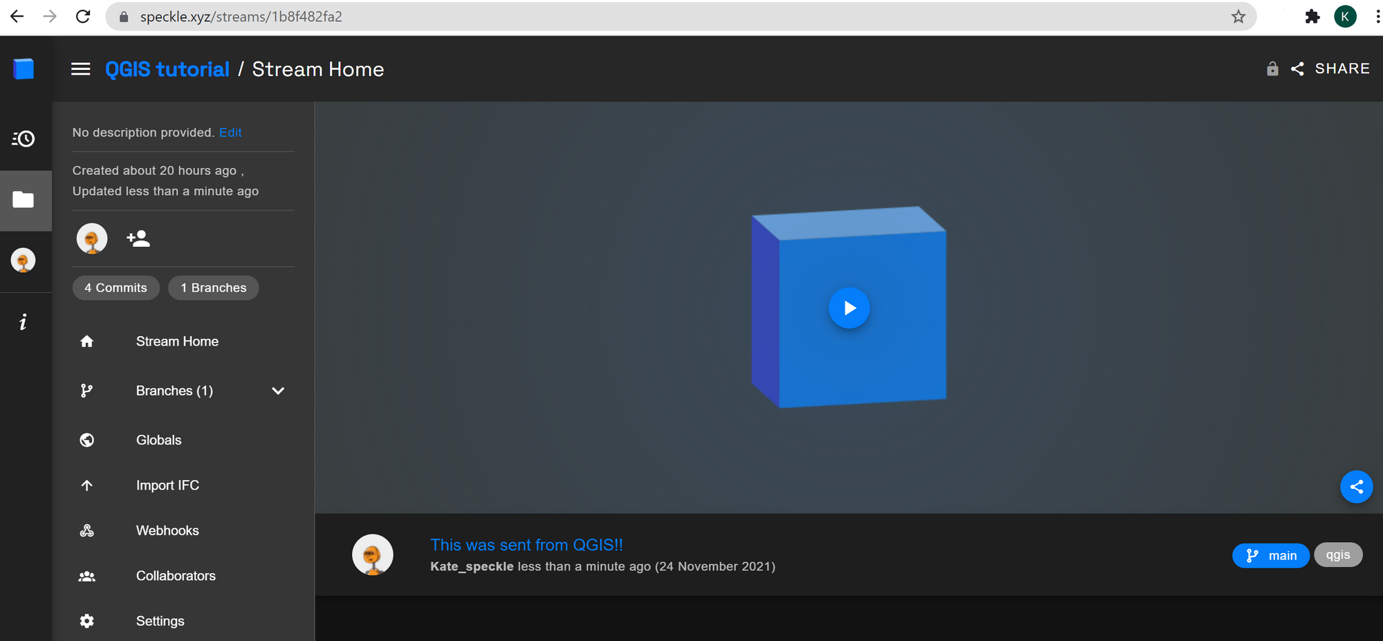
In your Stream page you should see a new commit created "less than a minute ago"! You can click on the blue title to open the page with this specific commit. This will be the URL you can use for receiving points later in Grasshopper, the format will be something like "https://speckle.xyz/streams/xxx/commits/xxx".
The last layer we would need is buildings layer. Let's open QuickOSM plugin again and use the query below: buildings (any), restricted by layer extent (our boundary). You can uncheck Lines, Multilinestrings and Points in Advanced tab. Click Run query.
Editing layer attributes
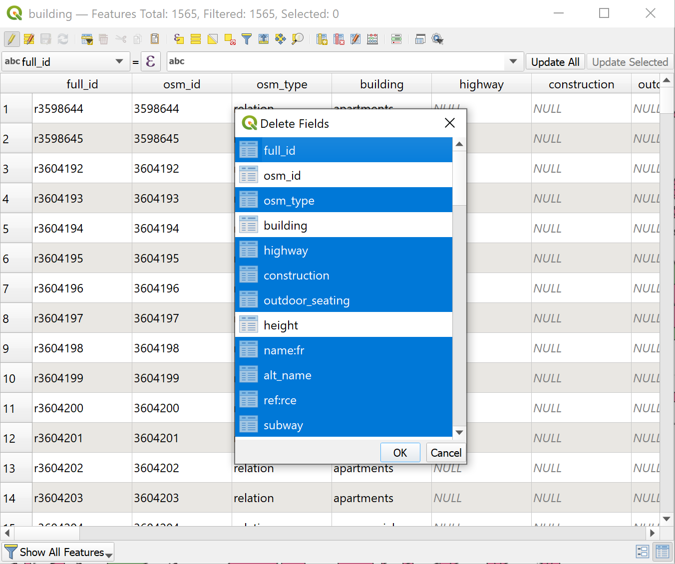
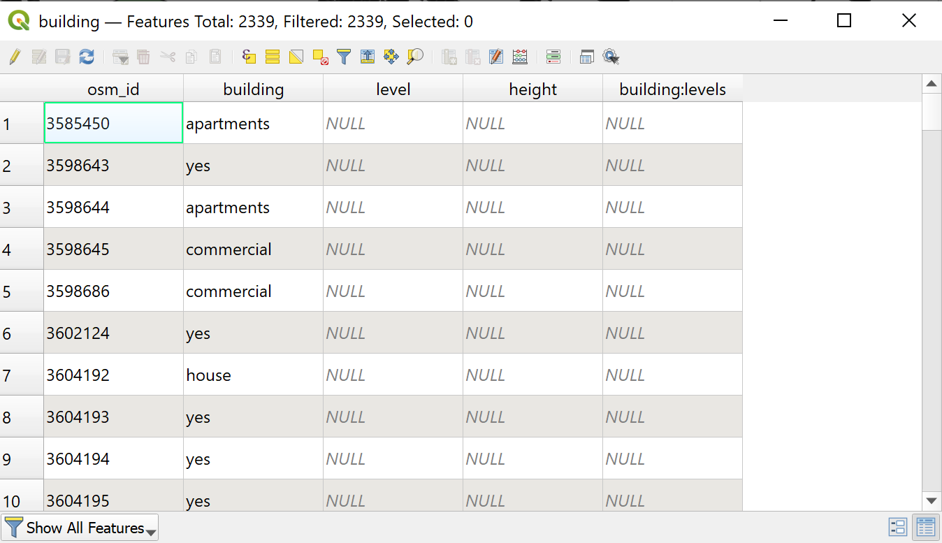
We have now a new layer "buildings" added. Usually OSM data has A LOT of attributes attached, so it would be good to filter out what's unnecessary before sending to Speckle. Let's open the Attribute table of the layer and activate editing mode (pencil icon). In the same panel you will see the button Delete field now activated, click on it. After selecting all fields you want to delete, click OK and then click again on a pencil icon to save edits. I left only 5 fields that might be necessary later.
Receiving data in Grasshopper
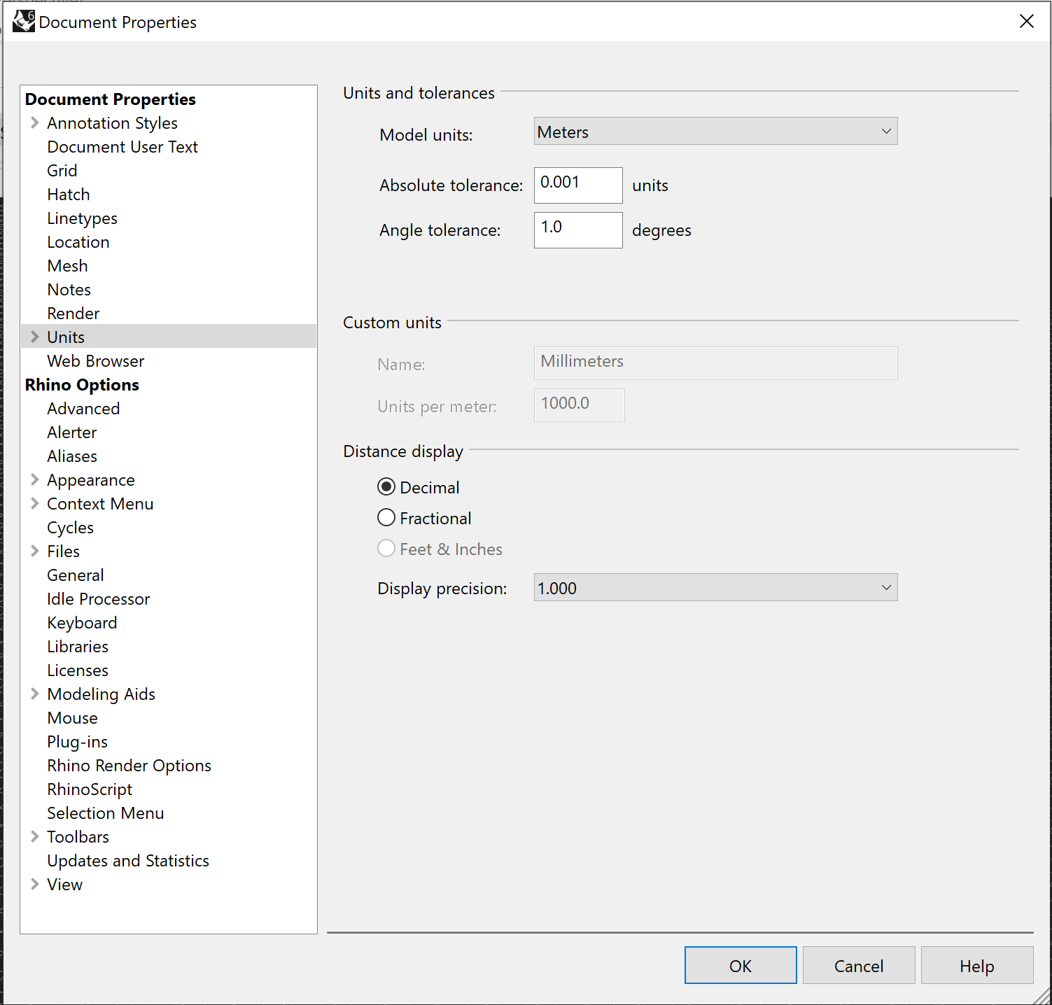
First, in Rhino File->Properties set Units to Meters.
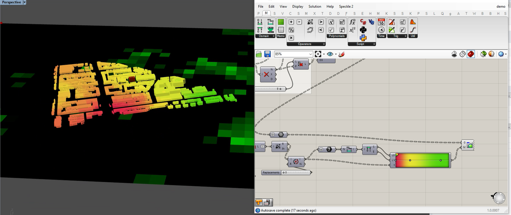
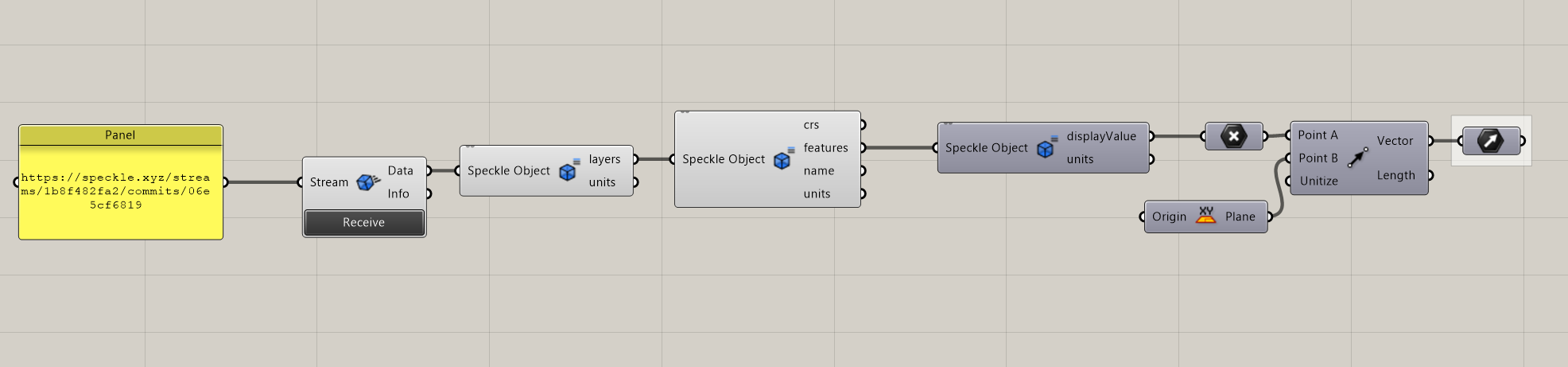
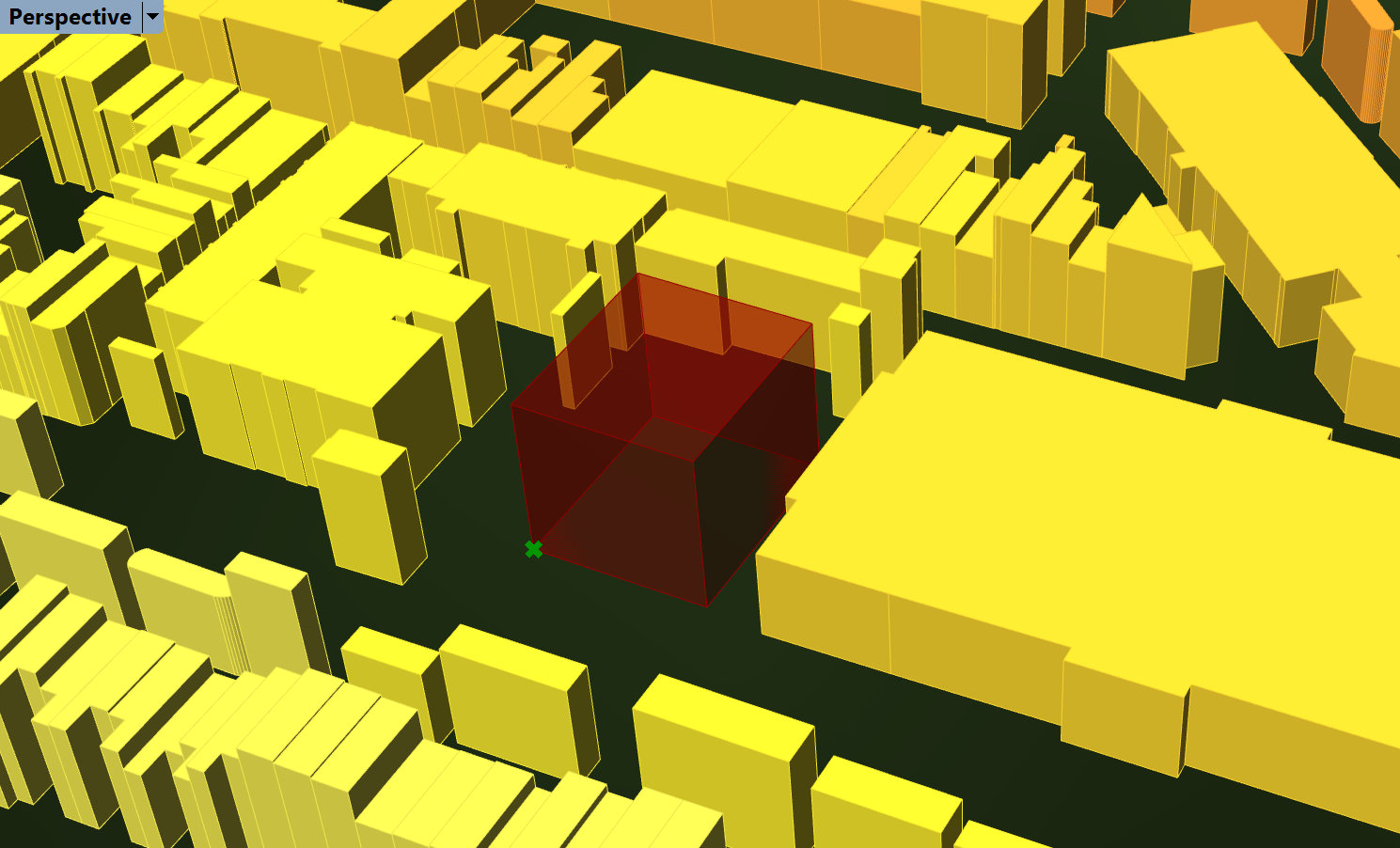
In Grasshopper find Speckle tab and the Receive component, set the commit URL where you sent the points, click Receive. Then, find the Expand Speckle Object component. You might need to add this component multiple times to get to the geometry (points, coded as "displayValue") and attached attributes. Select the last component, click the mouse wheel and select Zoom to focus Rhino's view on the points.
You can find the download link of the GH script in the end of the tutorial.
Cherry on top: adding survey point
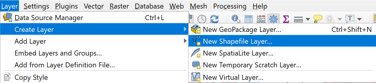
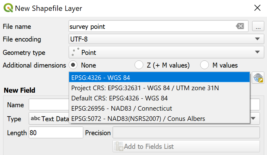
If you have a model in Rhino/Grasshopper with a point with known real world coordinates, you can create a point in QGIS to align geo-referenced data with your model later in Grasshopper. To do this, create a new shapefile layer of type Point in a geographic CRS, e.g. WGS 84.
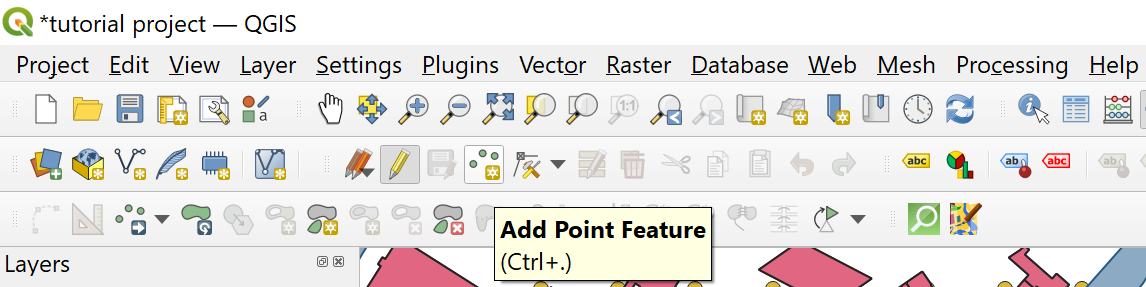
Activate editing mode (pencil) on Digitizing toolbar and click Add point feature. Place point somewhere on the canvas, assign id if required.
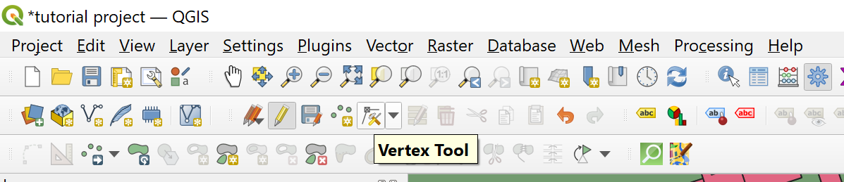
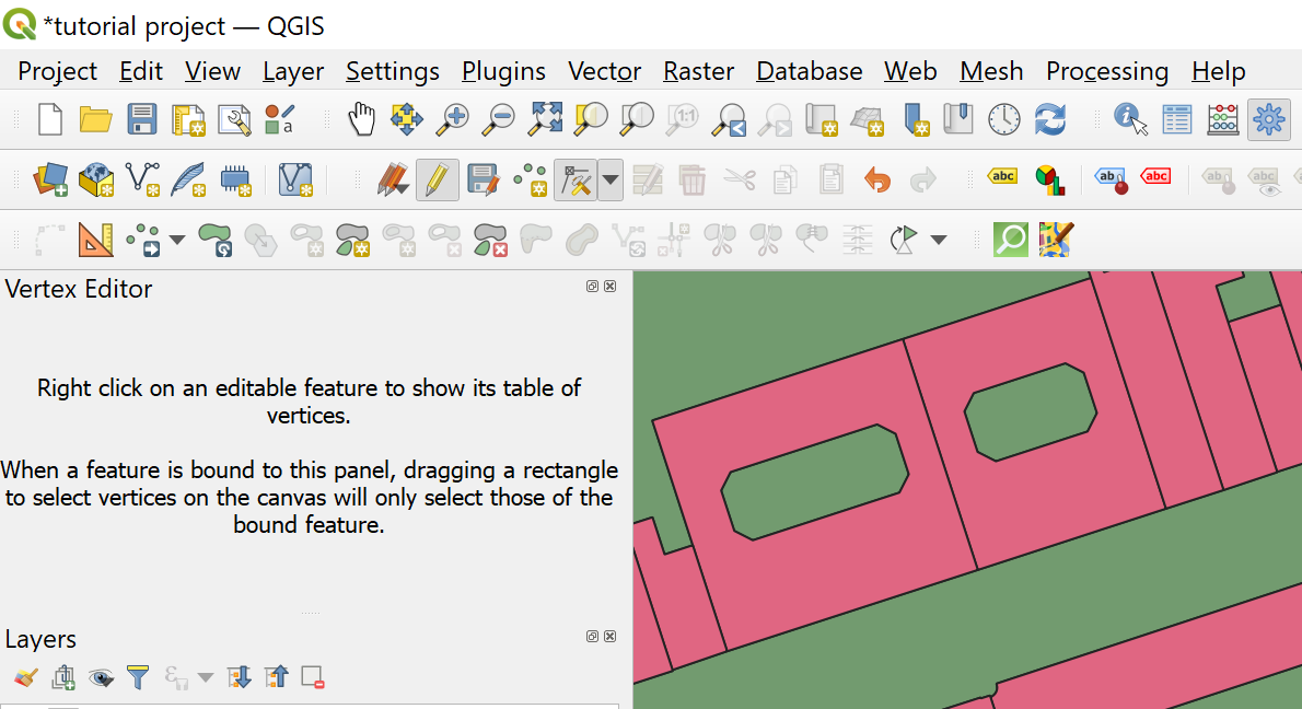
Select Vertex Tool. You will have a new toolbar opened on the side. As written on the panel, right-click on your new point.
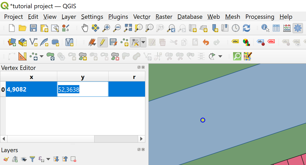
As you can see, the coordinates of the point are editable, you can set the correct ones and click pencil icon to save changes. Now reproject the layer to the same CRS as other layers and send to Speckle.
In Grasshopper you can create a vector directed to the plane origin, or to another point in the model which is based in the specified coordinates. You can use this vector to move all geometry received from QGIS to match your model.
Recap
Checklist for sending layers to Speckle:
- Set the Project CRS to Projected type
- Clean unnecessary attributes
Checklist for receiving layers in Grasshopper:
- Set Rhino units to meters
- Re-receive Speckle objects if they were created before units change
You can download full Grasshopper definition here.
Don't hesitate to ask any questions or suggestions that come to mind in the community forum!